If you want to make your work on Google Sheets look cleaner, there are various methods that you can try out. Google Sheets are similar to Microsoft’s Excel and it is a spreadsheet application for Google users. It can be used on both mobile and desktop. When presenting data on Google Sheets, one usually tries to make their work look cleaner and that can be done via wrapping.
In this article, we will discuss what is wrapping and the various methods that can be employed to use this shortcut or tool to make your work stand out.
Also read: How to create a table in Google Sheets?
Wrapping text
Google Sheets allows more than one user at a time to edit on Sheets, this way you can collaborate together and produce effective results. While working with someone or by yourself, you can try wrapping your data to make your spreadsheet presentation look cleaner.
Usually, if your data extends beyond one cell into the next or even the one after that, then your data will look uneven as some text might take two cells while others take up the space of three. To avoid this zig-zag outcome, you can wrap your text in one cell. This makes your work look clean and immaculate.
Given below are four wrapping methods that can help you wrap your data within one cell:
Use Format
You can use the format option to wrap up a row of your data that is overspilling out of one cell or even on individual cells. Follow the steps given below:
Step 1: Select all the cells that are to be wrapped. On the top, from the menu options click on Format
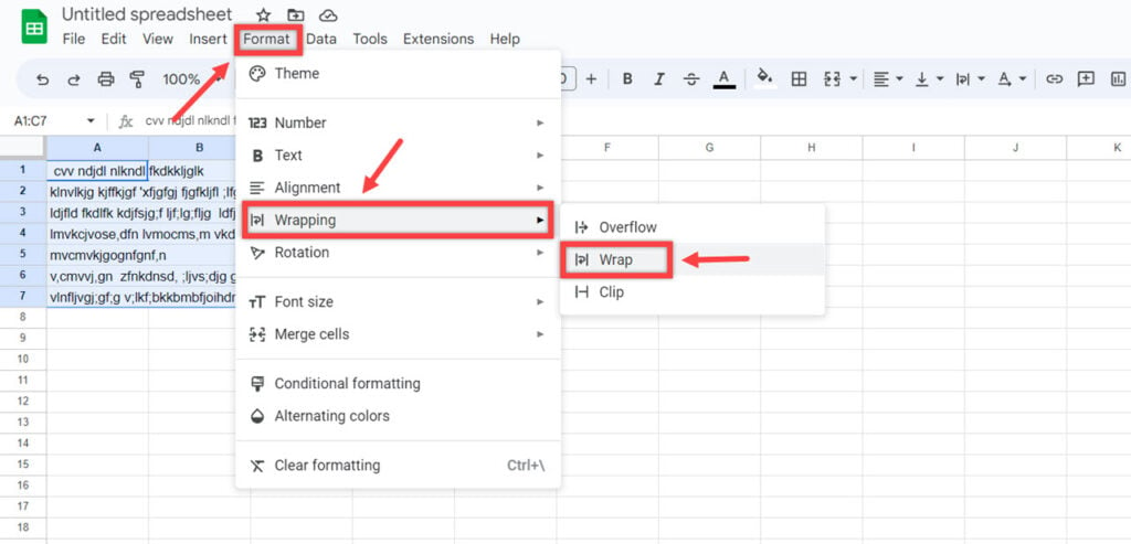
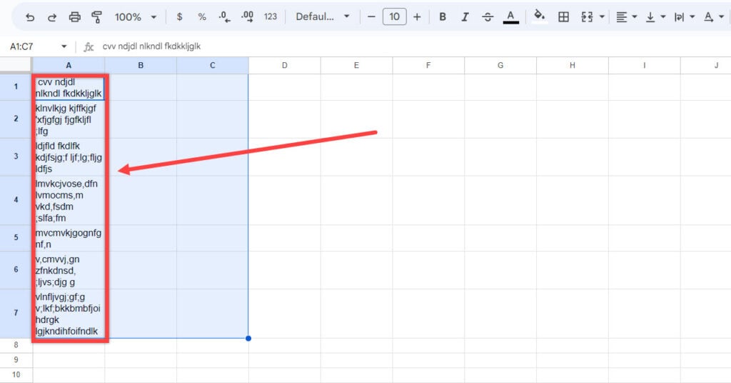
Step 2: Head to Wrapping from the drop-down options. Now click on Wrap. This will wrap up all the selected cells.
Also read: How to move a row in Excel?
Use Toolbar
Just below the menu on top, there is a toolbar that also has a wrapping icon. Select the row of cells or an individual cell that you would like to wrap and click on this icon. Choose Wrap from the options shown and viola!

Use Macros
Macros is short for macroinstruction which allows you to automate small repetitive tasks into keyboard shortcuts to save time. You can combine any task on Google Sheets with macros which can be achieved by simple keyboard shortcuts. In the example given below, we have combined the wrap tool with the keyboard shortcut: Ctrl + Alt + Shift + (choose any number). Now when you select a group of cells that need to be wrapped, you can press the shortcut buttons on the keyboard to wrap them.
You can use macros by following the steps given as follows:
Step 1: Head to the Extensions option in the menu on top and choose Macros from the drop-down options.

Step 2: Click on the Record macro option and then select the Use relative references option.

Step 3: Follow any of the two above-mentioned methods to wrap your text and then click on Save. Name your macro as ‘wrap text tool’ or anything of your preference and assign a number of your preference in front of the Ctrl + Alt + Shift + (choose any number) option and finally click on Save.

Now, whenever you are selecting a group of cells to wrap, you can head to either Extensions and Macros or you can press the given keyboard shortcut to wrap up the text in your cells.
Also read: How to add footnotes in Word?
Use Alt+Enter
Now this is not exactly applicable to a group of cells however, you can do this with individual cells. Choose the point in the sentence where you want to break it and click on that space. Now as the cursor hovers there, on your keyboard simultaneously press alt + enter keys to break the sentence. This will shift or wrap the rest of the sentence below the beginning of the sentence.

This keyboard shortcut can be specifically used after you have used the first three methods to create symmetry if there seems to be an uneven pattern of wrapping. This creates a very clear presentation of data or words. To undo the changes made by using this shortcut, you can press the undo button in the toolbar or backspace where the rest of the sentence was shifted below the beginning.

Also read: How to create a pie chart in Google Sheets?

